A decoder-only foundation model for time-series forecasting

Favorite

Posted by Rajat Sen and Yichen Zhou, Google Research

Time-series forecasting is ubiquitous in various domains, such as retail, finance, manufacturing, healthcare and natural sciences. In retail use cases, for example, it has been observed that improving demand forecasting accuracy can meaningfully reduce inventory costs and increase revenue. Deep learning (DL) models have emerged as a popular approach for forecasting rich, multivariate, time-series data because they have proven to perform well in a variety of settings (e.g., DL models dominated the M5 competition leaderboard).

At the same time, there has been rapid progress in large foundation language models used for natural language processing (NLP) tasks, such as translation, retrieval-augmented generation, and code completion. These models are trained on massive amounts of textual data derived from a variety of sources like common crawl and open-source code that allows them to identify patterns in languages. This makes them very powerful zero-shot tools; for instance, when paired with retrieval, they can answer questions about and summarize current events.

Despite DL-based forecasters largely outperforming traditional methods and progress being made in reducing training and inference costs, they face challenges: most DL architectures require long and involved training and validation cycles before a customer can test the model on a new time-series. A foundation model for time-series forecasting, in contrast, can provide decent out-of-the-box forecasts on unseen time-series data with no additional training, enabling users to focus on refining forecasts for the actual downstream task like retail demand planning.

To that end, in “A decoder-only foundation model for time-series forecasting”, we introduce TimesFM, a single forecasting model pre-trained on a large time-series corpus of 100 billion real world time-points. Compared to the latest large language models (LLMs), TimesFM is much smaller (200M parameters), yet we show that even at such scales, its zero-shot performance on a variety of unseen datasets of different domains and temporal granularities come close to the state-of-the-art supervised approaches trained explicitly on these datasets. Later this year we plan to make this model available for external customers in Google Cloud Vertex AI.

A decoder-only foundation model for time-series forecasting

LLMs are usually trained in a decoder-only fashion that involves three steps. First, text is broken down into subwords called tokens. Then, the tokens are fed into stacked causal transformer layers that produce an output corresponding to each input token (it cannot attend to future tokens). Finally, the output corresponding to the i-th token summarizes all the information from previous tokens and predicts the (i+1)-th token. During inference, the LLM generates the output one token at a time. For example, when prompted with “What is the capital of France?”, it might generate the token “The”, then condition on “What is the capital of France? The” to generate the next token “capital” and so on until it generates the complete answer: “The capital of France is Paris”.

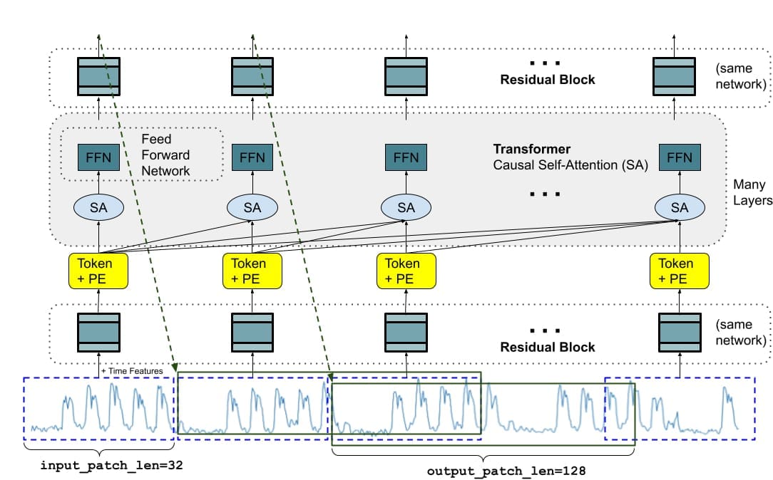
A foundation model for time-series forecasting should adapt to variable context (what we observe) and horizon (what we query the model to forecast) lengths, while having enough capacity to encode all patterns from a large pretraining dataset. Similar to LLMs, we use stacked transformer layers (self-attention and feedforward layers) as the main building blocks for the TimesFM model. In the context of time-series forecasting, we treat a patch (a group of contiguous time-points) as a token that was popularized by a recent long-horizon forecasting work. The task then is to forecast the (i+1)-th patch of time-points given the i-th output at the end of the stacked transformer layers.

However, there are several key differences from language models. Firstly, we need a multilayer perceptron block with residual connections to convert a patch of time-series into a token that can be input to the transformer layers along with positional encodings (PE). For that, we use a residual block similar to our prior work in long-horizon forecasting. Secondly, at the other end, an output token from the stacked transformer can be used to predict a longer length of subsequent time-points than the input patch length, i.e., the output patch length can be larger than the input patch length.

Consider a time-series of length 512 time-points being used to train a TimesFM model with input patch length 32 and output patch length 128. During training, the model is simultaneously trained to use the first 32 time-points to forecast the next 128 time-points, the first 64 time-points to forecast time-points 65 to 192, the first 96 time-points to forecast time-points 97 to 224 and so on. During inference, suppose the model is given a new time-series of length 256 and tasked with forecasting the next 256 time-points into the future. The model will first generate the future predictions for time-points 257 to 384, then condition on the initial 256 length input plus the generated output to generate time-points 385 to 512. On the other hand, if in our model the output patch length was equal to the input patch length of 32 then for the same task we would have to go through eight generation steps instead of just the two above. This increases the chances of more errors accumulating and therefore, in practice, we see that a longer output patch length yields better performance for long-horizon forecasting

TimesFM architecture.

Pretraining data

Just like LLMs get better with more tokens, TimesFM requires a large volume of legitimate time series data to learn and improve. We have spent a great amount of time creating and assessing our training datasets, and the following is what we have found works best:

Zero-shot evaluation results

We evaluate TimesFM zero-shot on data not seen during training using popular time-series benchmarks. We observe that TimesFM performs better than most statistical methods like ARIMA, ETS and can match or outperform powerful DL models like DeepAR, PatchTST that have been explicitly trained on the target time-series.

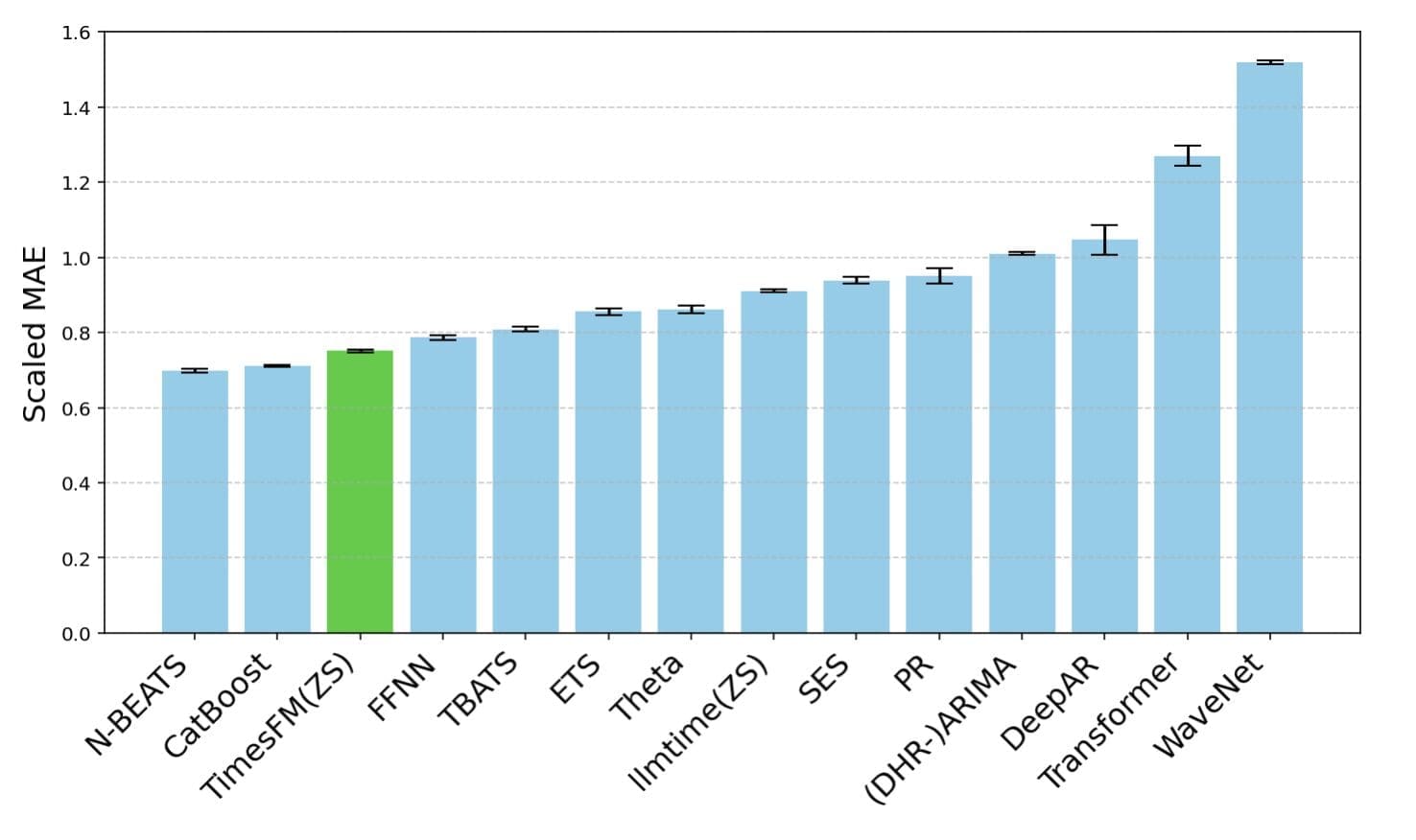
We used the Monash Forecasting Archive to evaluate TimesFM’s out-of-the-box performance. This archive contains tens of thousands of time-series from various domains like traffic, weather, and demand forecasting covering frequencies ranging from few minutes to yearly data. Following existing literature, we inspect the mean absolute error (MAE) appropriately scaled so that it can be averaged across the datasets. We see that zero-shot (ZS) TimesFM is better than most supervised approaches, including recent deep learning models. We also compare TimesFM to GPT-3.5 for forecasting using a specific prompting technique proposed by llmtime(ZS). We demonstrate that TimesFM performs better than llmtime(ZS) despite being orders of magnitude smaller.

Scaled MAE (the lower the better) of TimesFM(ZS) against other supervised and zero-shot approaches on Monash datasets.

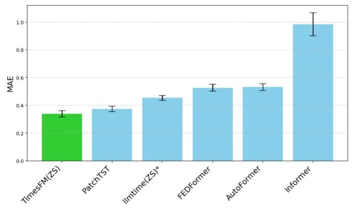
Most of the Monash datasets are short or medium horizon, i.e., the prediction length is not too long. We also test TimesFM on popular benchmarks for long horizon forecasting against a recent state-of-the-art baseline PatchTST (and other long-horizon forecasting baselines). In the next figure, we plot the MAE on ETT datasets for the task of predicting 96 and 192 time-points into the future. The metric has been calculated on the last test window of each dataset (as done by the llmtime paper). We see that TimesFM not only surpasses the performance of llmtime(ZS) but also matches that of the supervised PatchTST model explicitly trained on the respective datasets.

Last window MAE (the lower the better) of TimesFM(ZS) against llmtime(ZS) and long-horizon forecasting baselines on ETT datasets.

Conclusion

We train a decoder-only foundation model for time-series forecasting using a large pretraining corpus of 100B real world time-points, the majority of which was search interest time-series data derived from Google Trends and pageviews from Wikipedia. We show that even a relatively small 200M parameter pretrained model that uses our TimesFM architecture displays impressive zero-shot performance on a variety of public benchmarks from different domains and granularities.

Acknowledgements

This work is the result of a collaboration between several individuals across Google Research and Google Cloud, including (in alphabetical order): Abhimanyu Das, Weihao Kong, Andrew Leach, Mike Lawrence, Alex Martin, Rajat Sen, Yang Yang and Yichen Zhou.